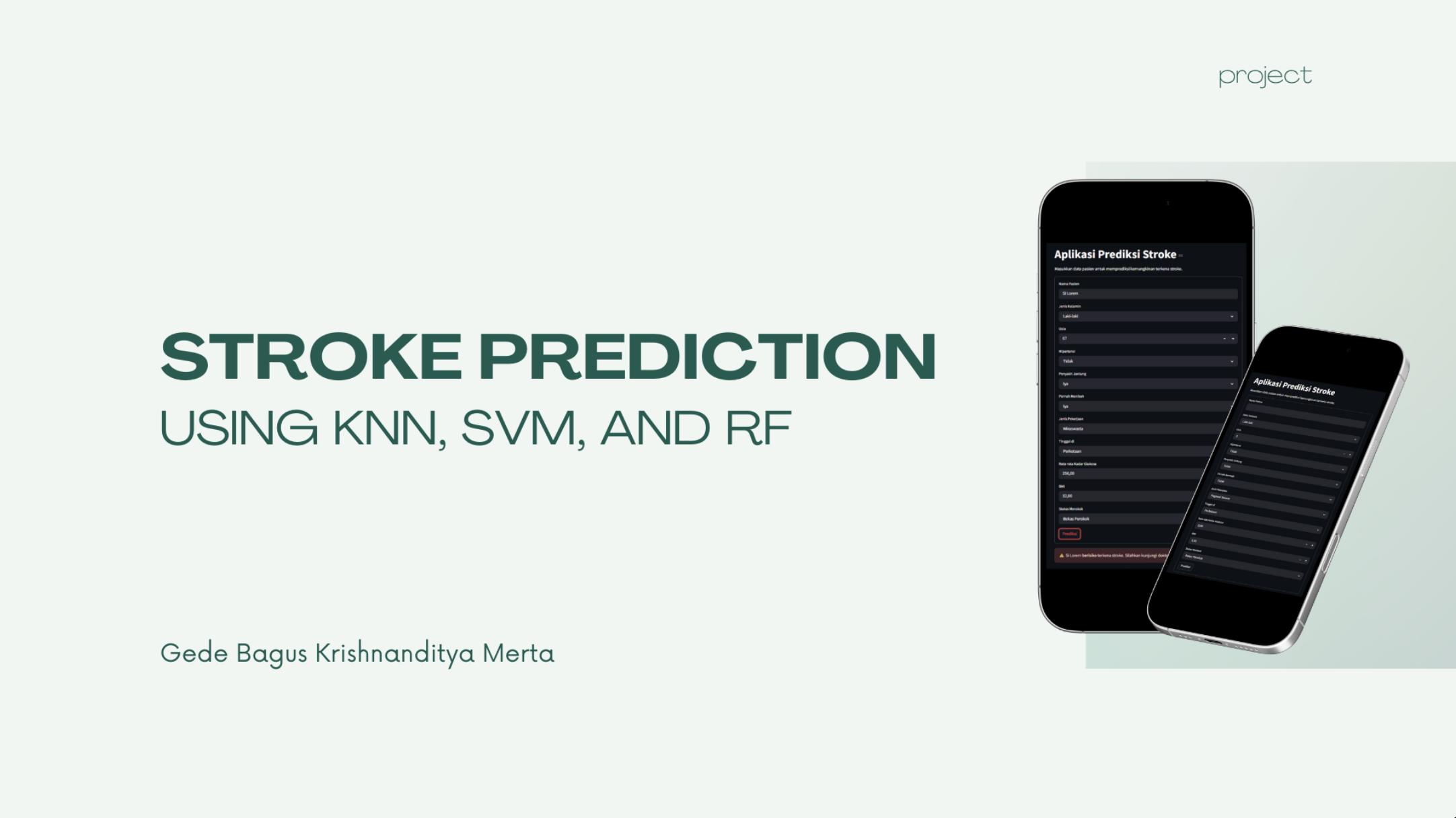
The Silent Pathology of Stroke
A stroke occurs when blood supply to part of the brain is suddenly cut off by an arterial blockage or a ruptured vessel. Deprived of oxygen and vital nutrients, brain cells begin to die within minutes. Globally, stroke is the second leading cause of death and a major contributor to long-term adult disability.
What makes stroke particularly dangerous is that its primary warning signs develop quietly. High blood pressure, elevated blood glucose, and obesity accumulate over years without causing daily pain or sudden disruptions. Routine health screenings record these biomarkers individually, but clinicians can miss how subtle multi-factor combinations quietly elevate a patient’s stroke probability.
For our Machine Learning capstone at Telkom University, my team and I wanted to see if statistical models could process routine health metrics to flag that hidden risk early.
When I first ran our baseline classifier on 5,110 patient records, the console printed a 95.1% accuracy score. For about ten seconds, my team and I thought our machine learning capstone was practically finished.
Then I opened the confusion matrix. The true positive count for stroke cases was exactly zero. The model had learned a simple, useless shortcut: because only 249 patients in the dataset had suffered a stroke (roughly 4.87%), predicting “no stroke” for every single person yielded 95.1% accuracy. In a clinical hospital ward, that model would miss 100% of at-risk patients while boasting an A-grade accuracy score.
Here is how I broke that false baseline and rebuilt the pipeline around clinical sensitivity.
Patient Health Records (5,110 Rows)
                 │
                 ▼
       Preprocessing Pipeline
   ├── Drop arbitrary 'id' column
   ├── Median imputation for missing BMI (~4%)
   ├── Outlier clipping on blood glucose & BMI
   └── Label / One-hot encoding
                 │
                 ▼
       The 95% Accuracy Trap
   (Predicts 0 for everyone -> Recall: 0.00)
                 │
                 ▼
     Class Imbalance Mitigation
   (SMOTE Oversampling on Train Folds Only)
                 │
                 ▼
   GridSearchCV with 5-Fold Stratified CV
   ├── SVM (RBF Kernel) -> Best overall
   ├── Random Forest -> Most interpretable
   └── KNN (Distance weighted)
                 │
                 ▼
    Streamlit Interactive Calculator
The Dataset and Missing Data Realities
The dataset contains 5,110 anonymized medical records across ten clinical and demographic features:
- Clinical measurements: age, hypertension (0 or 1), heart disease (0 or 1), average glucose level (mg/dL), and body mass index (BMI).
- Demographic variables: gender, ever married, work type, residence type, and smoking status.
- Target label: stroke (0 = no stroke, 1 = stroke).
Before touching any algorithms, the data had practical flaws. The id column was a database artifact that offered no predictive power, so I dropped it immediately.
BMI had missing values in about 4% of records (201 patients). Deleting those rows would throw away valuable clinical history, especially since several missing records belonged to the minority stroke class. Mean imputation is risky here because BMI distributions have long right tails from extreme obesity. I opted for median imputation, which preserves the central tendency without getting dragged by extreme outliers.
For numerical stability, I clipped extreme values in avg_glucose_level and bmi at the 99th percentile. Extreme laboratory values can distort distance-based classifiers like KNN, making distance calculations drift.
The Naive Approach: Falling for High Accuracy
With the data cleaned, I fed the features into a standard classifier without adjusting for class distribution. The training ran cleanly and holdout validation reported 95.13% accuracy.
Confusion Matrix (Naive Baseline):
                 Predicted No    Predicted Stroke
Actual No           4,861               0
Actual Stroke         249               0

Accuracy: 95.13%
Precision: 0.00
Recall:    0.00
F1-Score:  0.00
The classifier acted like a broken smoke detector that never rings because fires are rare. In medical screening, a false positive triggers an extra blood test or lifestyle consultation. A false negative sends an at-risk patient home with zero warning. Accuracy was entirely the wrong metric to optimize.
What happens if we force the model to treat stroke cases as equally important during training?
Balancing the Training Folds with SMOTE
To fix the imbalance, I applied Synthetic Minority Over-sampling Technique (SMOTE). Instead of duplicating minority rows, SMOTE creates synthetic points along the line segments connecting k-nearest neighbors within the minority class.
One critical rule guided this step: oversampling must only occur inside the training folds. If you apply SMOTE to the entire dataset before splitting, synthetic data points derived from test instances leak into your training set, inflating performance metrics with artificial data leakage.
I set up a 5-fold stratified cross-validation split, ensuring each fold kept the 4.87% stroke ratio, and applied SMOTE strictly to the four training folds in each iteration.
Comparing Three Classifiers
With balanced training folds, I ran grid searches across three distinct architectures to see how different decision boundaries handled clinical risk factors:
# Hyperparameter grids evaluated with GridSearchCV
svm_grid = {
    'C': [0.1, 1, 10, 100],
    'kernel': ['linear', 'rbf', 'poly'],
    'gamma': ['scale', 'auto']
}

rf_grid = {
    'n_estimators': [100, 200, 500],
    'min_samples_split': [2, 5, 10],
    'max_features': ['sqrt', 'log2']
}

knn_grid = {
    'n_neighbors': [3, 5, 7, 11],
    'weights': ['uniform', 'distance']
}
1. Support Vector Machine (RBF Kernel)
The radial basis function (RBF) kernel projects non-linear combinations of glucose, age, and blood pressure into higher dimensions.
- Optimal settings:
C = 10,gamma = 'auto',kernel = 'rbf' - Precision: 0.95
- Recall: 0.91
- F1-Score: 0.93
- Accuracy: 92.71%
SVM achieved the strongest balance. Setting C = 10 imposed a higher penalty on misclassified training points, pushing the margin away from stroke cases and keeping recall at 91%.
2. Random Forest
An ensemble of 200 trees provided clear feature importance rankings.
- Optimal settings:
n_estimators = 200,min_samples_split = 2 - Precision: 0.93
- Recall: 0.90
- F1-Score: 0.91
- Accuracy: 91.06%
Random Forest confirmed that age and average glucose level were the two strongest individual contributors to stroke risk in the dataset, matching medical literature.
3. K-Nearest Neighbors (KNN)
- Optimal settings:
n_neighbors = 3,weights = 'distance' - Precision: 0.97
- Recall: 0.79
- F1-Score: 0.87
- Accuracy: 87.95%
KNN produced an interesting trade-off: when it predicted a stroke, it was right 97% of the time (precision 0.97). However, its recall dropped to 0.79, meaning it missed 21% of real stroke cases. In clinical triage, missing one out of five at-risk patients is an unacceptable compromise.
Summary Benchmark
| Classifier | Best Parameters | Precision | Recall | F1-Score | Holdout Accuracy |
|---|---|---|---|---|---|
| SVM (RBF Kernel) | C=10, gamma='auto' | 0.95 | 0.91 | 0.93 | 92.71% |
| Random Forest | n_estimators=200, min_samples_split=2 | 0.93 | 0.90 | 0.91 | 91.06% |
| K-Nearest Neighbors | n_neighbors=3, weights='distance' | 0.97 | 0.79 | 0.87 | 87.95% |
SVM with an RBF kernel won on recall and F1-score. Its non-linear decision boundary separated subtle multi-factor risk combinations better than KNN’s local neighborhood votes.
Interactive Risk Calculator in Streamlit
To make these models testable beyond Jupyter notebooks, I wrapped the preprocessing pipeline and trained SVM model inside a Streamlit web application.
Clinician Enters 10 Health Metrics
               │
               ▼
   Streamlit Input Form
   (Age, Glucose, BMI, Hypertension, Habits)
               │
               ▼
   Preprocessing Pipeline
   (Imputation, Scaling, Encoding)
               │
               ▼
   Tuned SVM (RBF) Inference
               │
               ▼
   Risk Probability & Confidence Tier
A user fills in ten clinical fields, and the app runs feature encoding, median imputation, and SVM inference in real time, displaying the risk classification alongside a confidence score.
What I Learned
This project cured me of trusting headline accuracy metrics. A 95% accuracy score looks impressive on a slide, but when dealing with rare medical outcomes, it can hide complete predictive failure.
Class distribution dictates your loss function and evaluation strategy. Shifting our focus to recall and F1-score forced us to use SMOTE properly inside cross-validation folds, clip outliers that distorted distance metrics, and pick an RBF kernel that actually caught 91% of stroke cases.
The application remains an academic exploration on historical records, not a certified clinical instrument. But the engineering lesson is permanent: always check the confusion matrix before celebrating an accuracy number.